1	(Frequentist and Bayesian) Evaluation of Clinical Trial Designs Scott S. Emerson, M.D., Ph.D. Professor of Biostatistics, University of Washington
2	Course Structure Topics: Overview Frequentist approach Inferential methods Fixed Sample Clinical Trial Design Group Sequential Sampling Plans Evaluation of clinical trial designs Bayesian approach Inferential methods Probability models Nonparametric Bayes Evaluation of clinical trial designs
3
4
5
6	Overview Clinical Trial Setting
7	Fundamental Philosophy Statistics is about science. Science is about proving things to people. Other scientists Community at large
8	Scientific Studies A well designed study Discriminates between the most important, viable hypotheses Is equally informative for all possible outcomes Binary search using prior probability of being true Also consider simplicity of experiments, time, cost
9	Clinical Trials Experimentation in human volunteers Investigate a new treatment / preventive agent Safety Phase I; Phase II Efficacy Phase II (preliminary); Phase III Effectiveness Phase III (therapy); Phase IV (prevention)
10	Collaboration of Multiple Disciplines
11	Scientific Hypotheses Collaboration among investigators to Define intervention Define patient population Define general goal Clinical measurement for outcome Relevant benefit to establish: Two or more of Superiority, noninferiority, approximate equivalence, nonsuperiority, inferiority
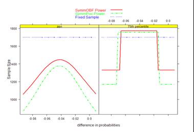
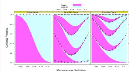
12	Typical Scientific Hypotheses The intervention when administered to the target population will tend to result in outcome measurements that are
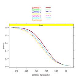
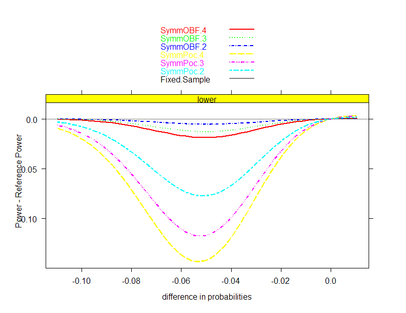
13	Experimental Design Plan collection of a sample which allows Administration of intervention (ethically) Measurement of outcomes Statistical analysis of results Variability of subjects means that results need to be reported in probabilistic terms Point estimate of summary measure of response Interval estimate to quantify precision Quantification of error rates for decisions (Binary decision?)
14	Refining Scientific Hypotheses In order to be able to perform analysis Modify intervention, endpoints to increase precision (without changing relevance) Probability model for response Choose summary measure of response distribution Precise statement of hypotheses to be discriminated Stated in terms of summary measure
15	Comparison of Summary Measures Typical approaches to compare response across two treatment arms Difference / ratio of means (arithmetic, geometric, …) Difference / ratio of medians (or other quantiles) Median difference of paired observations Difference / ratio of proportion exceeding some threshold Ratio of odds of exceeding some threshold Ratio of instantaneous risk of some event (averaged across time?) Probability that a randomly chosen measurement from one population might exceed that from the other …
16	Statistical Models Issues when choosing statistical models Criteria for quantifying credibility of results Frequentist Bayesian Computational methods and formulas Covariate adjustment …
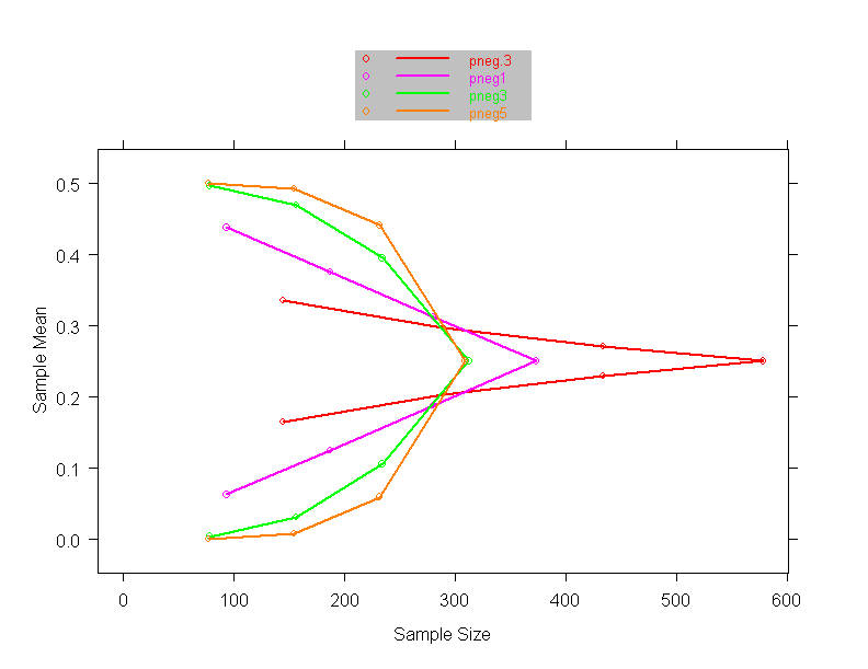
17	Impact of Statistical Model Choice of statistical model impacts the scientific question actually addressed as well as the statistical precision Robustness of inference depends on methods of computing the summary measures to be compared Interpretation of positive and negative studies depends on computation of sampling variance
18	Overview Where I Am Going: “A revolution no one will notice”
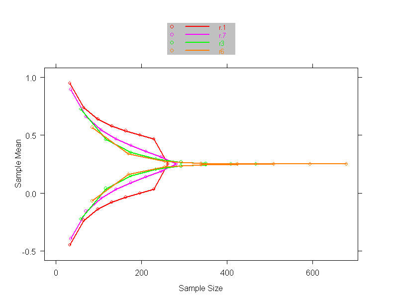
19	Ultimate Goal Design and analysis of clinical trials to allow quantification of the strength of evidence for or against scientific hypotheses AND to allow concise presentation of results Need to convince the audience, who may Disagree on what are most important hypotheses What precision is necessary for what endpoints? Disagree on definition of statistical evidence Frequentist vs Bayesian (with varying priors)
20	My Optimality Criterion I believe statistical methods should always take the scientific setting into account Science ideally progresses through a series of experiments successively addressing more refined questions I am against unnecessarily assuming the answer to more detailed questions than I am trying to address in the scientific study
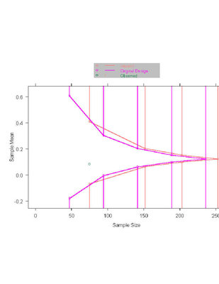
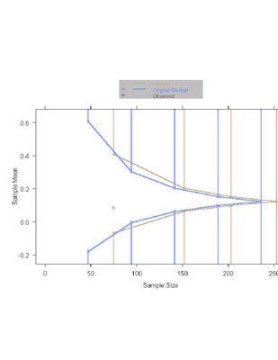
21	"There are two types of..." There are two types of people in the world: Those who dichotomize everything, and Those who don’t.
22	Classification of Statistical Models Breiman (2000): The two approaches to data analysis Model based vs algorithmic (e.g., regression vs trees, neural nets) This talk: Frequentist vs Bayesian (Semi)Parametric vs nonparametric
23	Outline Frequentist Methods Frequentist inference in fixed sample designs Probability models (Semi)parametric vs nonparametric Sequential sampling Bayesian Methods Bayesian paradigm “Coarsened” nonparametric Bayes Concise presentation of results
24	Frequentist Methods Frequentist Inference in Fixed Sample Designs
25	Illustrative Example Hypothetical clinical trial Two groups: Treatment and Placebo Primary outcome variable: continuous Notation
26	Measure of Treatment Effect We choose some summary measure of the difference between the distributions of response across the treatment arms Criteria (in order of importance) Scientifically (clinically) relevant Also reflects current state of knowledge Intervention is likely to affect Could be based on ability to detect variety of changes Statistical precision
27	Measure of Treatment Effect A common choice: Difference in means Why? Occasionally most relevant (health care costs) Sensitive to a wide variety of changes in distribution of response Statistically most efficient in the presence of normally distributed data
28	Statistical Design of Experiment Design experiment by looking to the future: Consider how the results of the study will be reported The single “best” estimate of treatment effect An interval estimate to quantify precision A quantification of the strength of evidence for or against particular hypotheses Our conclusion from the study A binary decision
29	One-sided Statistical Hypotheses Define hypotheses to be discriminated Decisions for superiority or not sufficiently superior (One-sided test can also be defined for one-sided lesser alternative)
30	Two-sided Statistical Hypotheses Define hypotheses to be discriminated Resembles two superposed one-sided tests Decisions for superiority, inferiority, approximate equivalence
31	Classical Hypothesis Testing Reject hypothesis if observed data is rare when that hypothesis is true Consider probability of falsely rejecting each hypothesis Usually fix type I error at some prescribed level Try for high power (low type II error) for some “design alternative”
32	Implementation Define “rare data” for each hypothesis Choose test statistic Often based on an estimate of treatment effect Reject low treatment effect when estimate is so high as to only occur, say, with 5% probability
33	Hallmark of Frequentist Inference Frequentist inference makes probability statements about the distribution of the data conditional on a presumed treatment effect, e.g.,
34	Sampling Distribution Frequentist inference thus requires knowledge of the sampling distribution for the estimate of treatment effect Sampling distribution under the null Necessary and sufficient to have the correct size test Sampling distribution under alternatives Necessary to compute power of tests confidence intervals optimality of estimators
35	Derivation of Sampling Distribution To compute sampling distribution need to know the probability model to obtain Formula for Definition of hypotheses Distribution of under every hypothesis
36	Typical Sampling Distribution In the probability models most often used for frequentist inference, the sampling distribution is approximately normal Fixed sample setting (no early stopping) Large samples
37	Approximate Frequentist Inference Standard frequentist inference is then Consistent point estimate 100(1-α)% confidence interval P value to test
38	Frequentist Methods Sample Size Determination
39	Decision Theoretic Approach Design study with sufficient precision to be able to reject at least one hypothesis with high confidence Equivalent criteria for rejection type I error = type II error interval estimate does not contain both the null and alternative hypotheses Asymmetric definitions of rejection Arbitrary power
40	Sample Size Computation Number of “sampling units” to obtain desired precision
41	When Sample Size Constrained Often (usually?) logistical constraints impose a maximal sample size Compute power to detect specified alternative Compute alternative detected with high power
42	Threshold for Statistical Significance Having chosen a sample size, we can compute Threshold for declaring statistical significance
43	Inference at Threshold We can also anticipate the inference we will make if we observe an estimate exactly at the threshold P value equal to type I error Confidence interval
44	Frequentist Methods Evaluation of Fixed Sample Clinical Trial Designs
45	Evaluation of Designs Process of choosing a trial design Define candidate design Usually constrain two operating characteristics Type I error, power at design alternative Type I error, maximal sample size Evaluate other operating characteristics Different criteria of interest to different investigators Modify design Iterate
46	Operating Characteristics Frequentist power curve Type I error (null) and power (design alternative) Sample size requirements Threshold for statistical significance Frequentist inference at threshold Point estimate Confidence interval P value
47	Collaboration of Multiple Disciplines
48	Evaluating Sample Size Consider Feasibility of accrual Credibility of results “3 over n rule”: We may have missed an important subgroup with different response patterns When combined with results from earlier trials
49	Evaluating Power Curve Probability of rejecting null for arbitrary alternatives Type I error (power under null) Power for specified alternative Alternative rejected by design Alternative for which study has high power Interpretation of negative studies
50	Evaluating Boundaries Threshold for declaring statistical significance On the scale of estimated treatment effect Assess clinical importance Assess economic importance
51	Evaluating Inference Inference on the boundary for statistical significance Frequentist Point estimates Confidence intervals P values
52	Frequentist Methods Sequential Sampling: Stopping Rules
53	Statistical Design: Sampling Plan Ethical and efficiency concerns are addressed through sampling which might allow early stopping During the conduct of the study, data are analyzed and reviewed at periodic intervals Using interim estimates of treatment effect Decide whether to continue the trial If continuing, decide on any modifications to sampling scheme
54	Criteria for Early Stopping Results convincing for specific hypotheses Superiority, approximate equivalence, inferiority Results suggestive of inability to ultimately establish a hypothesis of interest Futility No advantage in continuing No need to collect additional data on safety, longer term follow-up, other secondary endpoints
55	Basis for Early Stopping Extreme estimates of treatment effect Curtailment: Boundary reached early Stochastic Curtailment: High probability that a particular decision will be made at final analysis Group sequential test: Formal decision rule in classical frequentist framework controlling experimentwise error Bayesian analysis: Posterior probability of hypothesis is high
56	General Stopping Rule Analyses when sample sizes N₁,…, N_J Can be randomly determined At jth analysis choose stopping boundaries a_j < b_j < c_j < d_j Compute test statistic T(X₁,…, X_N_j) Stop if T < a_j (extremely low) Stop if b_j < T < c_j (approximate equivalence) Stop if T > d_j (extremely high) Otherwise continue (with possible adaptive modification of analysis schedule, sample size, etc.)
57	Categories of Sequential Sampling Prespecified stopping guidelines Adaptive procedures
58	Prespecified Stopping Plans Prior to first analysis of data, specify Rule for determining maximal statistical information E.g., fix power, maximal sample size, or calendar time Rule for determining schedule of analyses E.g., according to sample size, statistical information, or calendar time Rule for determining conditions for early stopping E.g., boundary shape function for stopping boundaries on the scale of some test statistic
59	Boundary Scales A stopping rule for one test statistic is easily transformed to a stopping rule for another “Group sequential stopping rules” Sum of observations Point estimate of treatment effect Normalized (Z) statistic Fixed sample P value Error spending function Conditional probability Predictive probability Bayesian posterior probability
60	Families of Stopping Rules Parameterization of boundary shape functions facilitates search for stopping rules Can be defined for any boundary scale
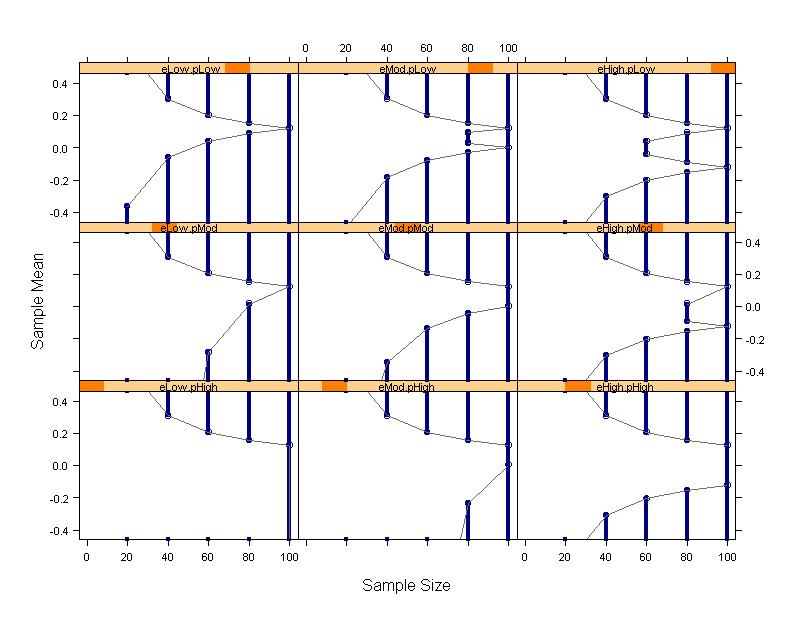
61	Example: Unified Family Down columns: Early vs no early stopping Across rows: One-sided vs two-sided decisions
62	Example: Unified Family A wide variety of boundary shapes possible All of the rules depicted have the same type I error and power to detect the design alternative
63	Adaptive Sampling Plans At each analysis of the data, the sampling plan can be modified to account for changed perceptions of possible results E.g., Proschan & Hunsberger (1995) Use conditional power considerations to modify ultimate sample size E.g., Self-designing Trial (Fisher, 1998) Prespecify weighting of groups “just in time” Weighting for each group only need be specified at immediately preceding analysis
64	Adaptive Sampling: The Price Adaptive sampling plans are less efficient Tsiatis & Mehta (2002) A classic prespecified group sequential stopping rule can be found that is more efficient than a given adaptive design Shi & Emerson (2003) Fisher’s test statistic in the self-designing trial provides markedly less precise inference than that based on the MLE To compute the sampling distribution of the latter, the sampling plan must be known
65	Prespecified Sampling: The Price Full knowledge of the sampling plan is needed to assess the full complement of frequentist operating characteristics In order to obtain inference with maximal precision and minimal bias, the sampling plan must be well quantified (Note that adaptive designs using ancillary statistics pose no special problems if we condition on those ancillary statistics.)
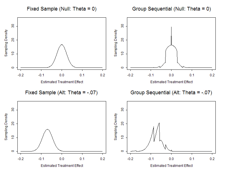
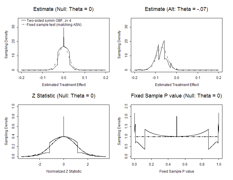
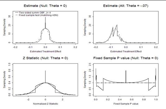
66	Major Issue: Frequentist Inference Frequentist operating characteristics are based on the sampling distribution Stopping rules do affect the sampling distribution of the usual statistics MLEs are not normally distributed Z scores are not standard normal under the null (1.96 is irrelevant) The null distribution of fixed sample P values is not uniform (They are not true P values)
67	Sampling Distribution of Estimates
68	Sampling Distribution of Estimates
69	Sampling Distributions of Statistics
70	Operating Characteristics For any stopping rule we can compute the correct sampling distribution and obtain Power curves Sample size distribution Bias adjusted estimates Correct (adjusted) confidence intervals Correct (adjusted) P values Candidate designs can then be compared with respect to their operating characteristics
71	Sequential Sampling Issues Design stage Satisfy desired operating characteristics E.g., type I error, power, sample size requirements Monitoring stage Flexible implementation of the stopping rule to account for assumptions made at design stage E.g., sample size adjustment to account for observed variance Analysis stage Providing inference based on true sampling distribution of test statistics
72	Bottom Line “You better think (think) think about what you’re trying to do…” - Aretha Franklin
73	Frequentist Methods Evaluation of Group Sequential Clinical Trial Designs
74	Case Study: Clinical Trial In Gm- Sepsis Randomized, placebo controlled Phase III study of antibody to endotoxin Intervention: Single administration Endpoint: Difference in 28 day mortality rates Placebo arm: estimate 30% mortality Treatment arm: hope for 23% mortality Analysis: Large sample test of binomial proportions Frequentist based inference Type I error: one-sided 0.025 Power: 90% to detect θ < -0.07 Point estimate with low bias, MSE; 95% CI
75	Evaluation of Designs Process of choosing a trial design Define candidate design Usually constrain two operating characteristics Type I error, power at design alternative Type I error, maximal sample size Evaluate other operating characteristics Different criteria of interest to different investigators Modify design Iterate
76	Operating Characteristics Same general operating characteristics of interest no matter the type of stopping rule Frequentist power curve Type I error (null) and power (design alternative) Sample size requirements Maximum, average, median, other quantiles Stopping probabilities Inference at each boundary Frequentist point estimate, confidence interval, P value Futility measures Conditional power, predictive power
77	Evaluating Sample Size Sample size a random variable Summary measures of distribution as a function of treatment effect maximum (feasibility of accrual) mean (Average Sample N- ASN) median, quartiles Stopping probabilities Probability of stopping at each analysis as a function of treatment effect Probability of each decision at each analysis
78	Evaluating Power Curve Probability of rejecting null for arbitrary alternatives Level of significance (power under null) Power for specified alternative Alternative rejected by design Alternative for which study has high power Interpretation of negative studies
79	Case Study: Boundaries and Power Curves O’Brien-Fleming, Pocock boundary shape functions when J= 4 analyses and maintain power
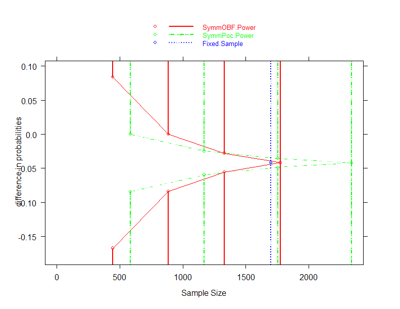
80	Case Study: Impact of Interim Analyses Required increased maximal sample size in order to maintain power Maximal sample size with 4 analyses O’Brien-Fleming: N= 1773 ( 4.3% increase) Pocock : N= 2340 (37.6% increase) Need to consider Average sample size Probability of continuing past 1700 subjects Conditions under which continue past 1700 subjects
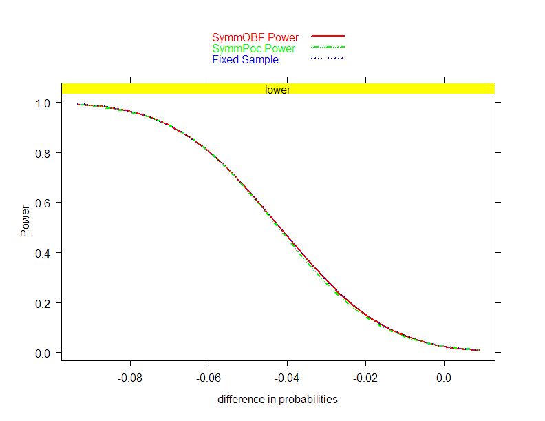
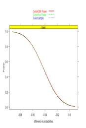
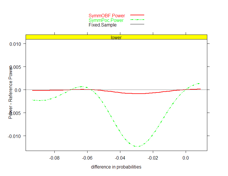
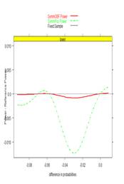
81	Case Study: ASN, 75^th %tile of Sample Size O’Brien-Fleming, Pocock boundary shape functions;J=4 analyses and maintain power
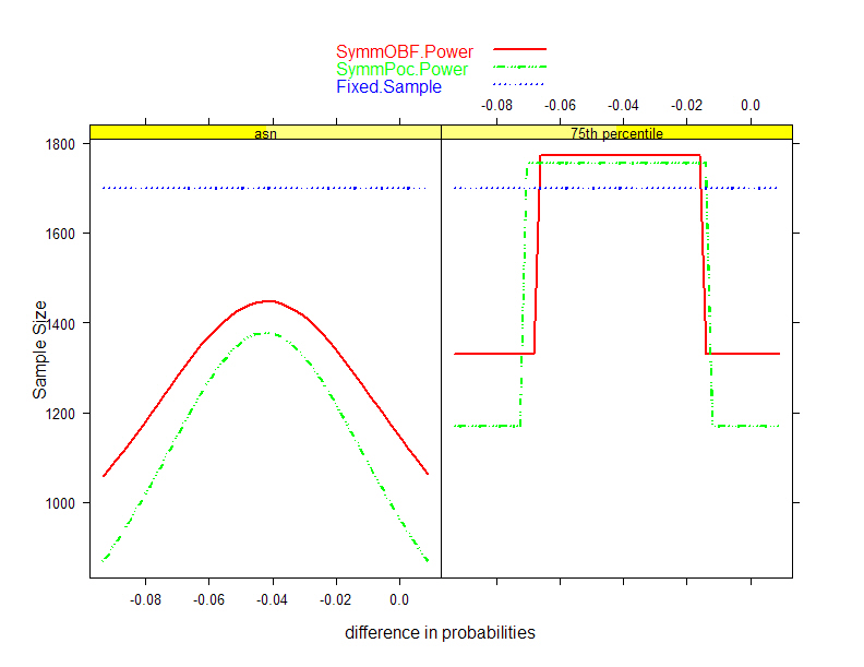
82	Case Study: Cumulative Stopping Probabilities O’Brien-Fleming, Pocock boundary shape functions when J=4 analyses and maintain power
83	Case Study: Impact of Interim Analyses Increased maximal sample size actually afforded better efficiency on average Pocock boundary shape function: lower ASN over range of alternatives examined This improved behavior despite the 36.7% increase in maximal sample size Worst case behavior O’Brien-Fleming: never more than N= 1773 Pocock continues past 1755 only if MLE for treatment effect is between -0.0357 and -0.0488 Always less than 16.01% chance, which occurs when the difference in mortality is -0.0422
84	Case Study: Sponsor’s Preferences Sponsor preferred not to increase maximal sample size beyond N= 1700 When investigating the boundaries, the sponsor was surprised to find that a difference of -0.042 would be statistically significant No one had informed the clinical and management teams of the boundary for the fixed sample test Such an effect was only of borderline clinical importance
85	Case Study: Power Curves: Maintain N OBF, Poc boundary shape functions when J= 2, 3, or 4 analyses and maintain N = 1700
86	Evaluating Boundaries Stopping boundary at each analysis On the scale of estimated treatment effect Inform DMC of precision Assess ethics May have prior belief of unacceptable levels Assess clinical, economic importance On the Z, fixed sample P value, or error spending scales
87	Case Study: Tabled boundaries on MLE Scale
88	Evaluating Inference Inference on the boundary at each analysis Frequentist Adjusted point estimates Adjusted confidence intervals Adjusted P values
89	Case Study: Inference on the Boundaries
90	Evaluating Futility Probability that a different decision would result if trial continued Compare unconditional power to fixed sample test with same sample size Conditional power Assume specific hypotheses Assume current best estimate Predictive power Assume Bayesian prior distribution
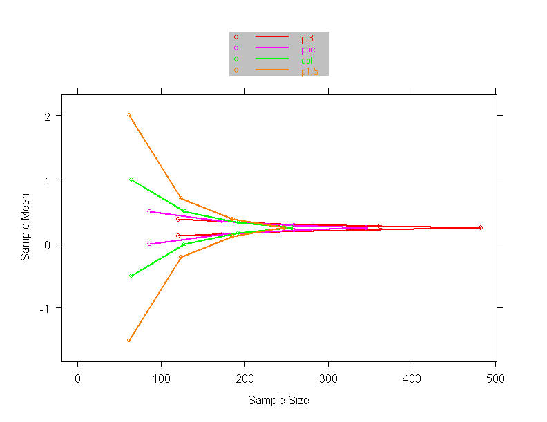
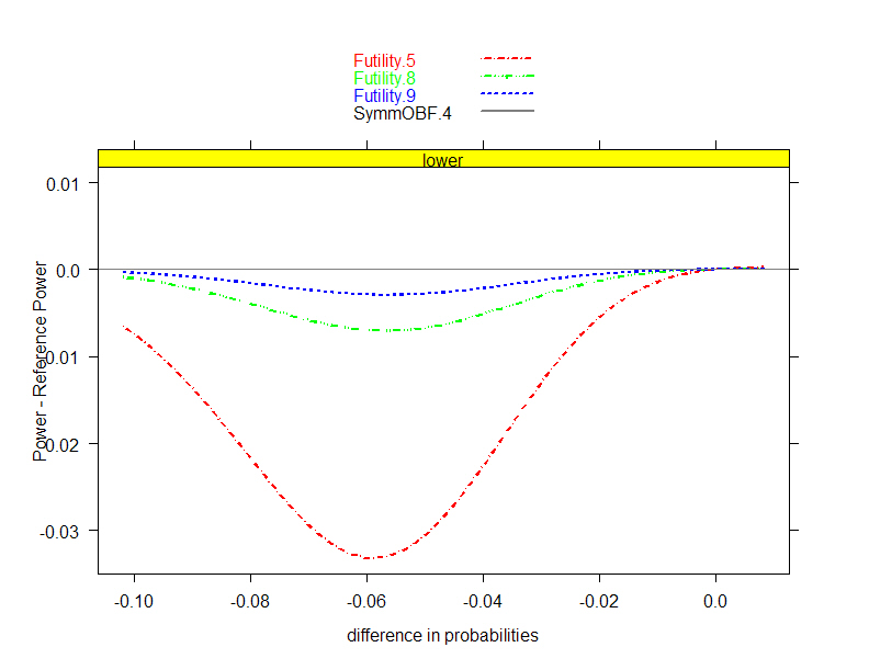
91	Case Study: Futility Boundary Sponsor desired greater efficiency when treatment effect is low Explored asymmetric designs with a range of boundary shape functions from unified family P= 0.5 (Pocock), 0.8, 0.9, 1.0 (O’Brien-Fleming) Compare unconditional power and ASN curves Rationale: Are we losing power by stopping early? If not, then we are not making bad futility decisions on average
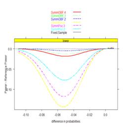
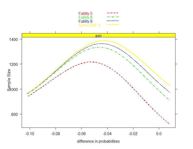
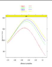
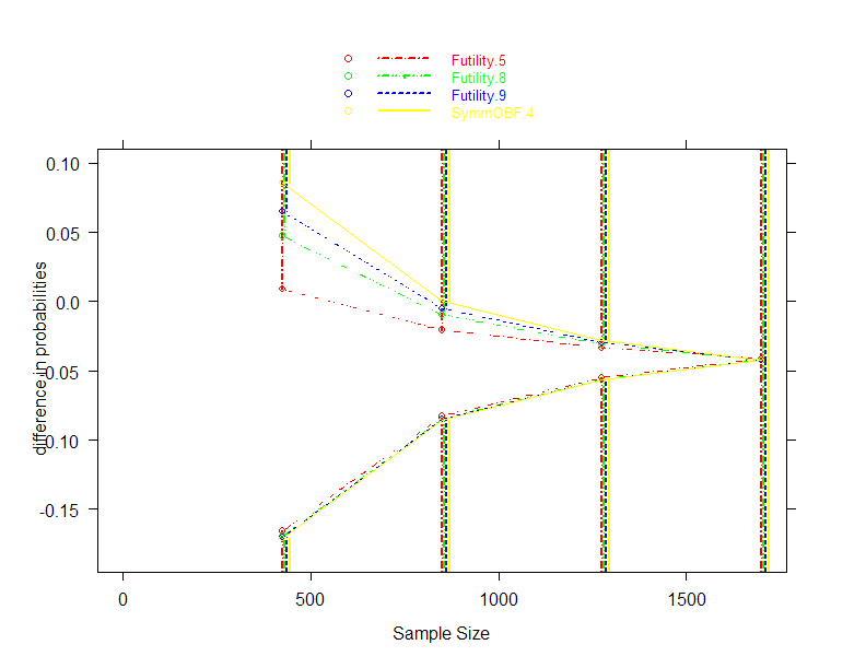
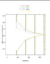
92	Case Study: Boundaries, Power, ASN Curves O’Brien-Fleming efficacy, spectrum of futility boundaries; J= 4 analyses and N=1700 Power Boundaries (Relative to Symmetric OBF) ASN
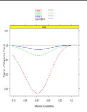
93	Case Study: Sponsor’s Futility Boundary Sponsor opted for futility boundary based on P= 0.8 Power – ASN tradeoff Worst case loss of power .0071 (from 0.738 to 0.731 when difference in mortality is -0.0566) 10.2% gain in average efficiency under null (ASN from 1099 to 987 when difference in mortality is 0.00)
94	Case Study: Stochastic Curtailment We are sometimes asked about stochastic curtailment Boundaries can be expressed on conditional power and predictive power scales Conditional power: Probability of later reversing the potential decision at interim analysis by conditioning on interim results and presumed treatment effect Predictive power: Like conditional power, but use a Bayesian prior for the presumed treatment effect
95	Case Study: Stochastic Curtailment Key issue: Computations are based on assumptions about true treatment effect Conditional power “Design”: assume hypothesis being rejected (assumes observed data is relatively misleading) “Estimate”: assume that current data is representative (assumes observed data is exactly accurate) Predictive power “Prior assumptions”: Use Bayesian prior distribution “Sponsor”: Centered at -0.07; plus/minus SD of 0.02 “Noninformative”
96	Case Study: Boundaries on Futility Scales
97	Case Study: Education of DMC, Sponsor Very different probabilities based on assumptions about true treatment effect Extremely conservative O’Brien-Fleming boundaries correspond to conditional power of 50% (!) under alternative rejected by the boundary Resolution of apparent paradox: if the alternative were true, there is less than .0001 probability of stopping for futility at the first analysis
98	Stochastic Curtailment Comments Neither conditional power nor predictive power have good foundational motivation Frequentists should use Neyman-Pearson paradigm and consider optimal unconditional power across alternatives Bayesians should use posterior distributions for decisions
99	Stochastic Curtailment Comments My experience I have consulted with many researchers on successive clinical trials Often I am asked about stochastic curtailment the first time Never have I been asked about it on the second trial
100	Evaluating Marketable Results Probability of obtaining estimates of treatment effect with clinical (and therefore marketing) appeal Modified power curve Unconditional Conditional at each analysis Predictive probabilities at each analysis
101	Case Study: Marketability Potential to have statistically significant treatment effect estimate of -0.06 or better O’Brien-Fleming efficacy boundary at third analysis: Terminate if bias adjusted estimate -0.055 or better What is the chance of obtaining -0.06 or better at the fourth analysis if study continues? If true effect is -0.07, probability of 4.1% of BAM < -0.06 If true effect is -0.06, probability of 3.6% of BAM < -0.06
102	Case Study: Modification for Marketability Modify third analysis efficacy boundary to correspond to BAM of -0.06 or better Probability of BAM < -0.06 increases If true effect is -0.07: from 66.6% to 68.6% If true effect is -0.06: from 50.4% to 54.0%
103	Final Comments Adaptive designs versus prespecified stopping rules Adaptive designs come at a price of efficiency With careful evaluation of designs, there is little need for adaptive designs Everything I showed today was known prior to collecting any data in the clinical trial Prespecified stopping rules can be chosen which find best tradeoffs among the various collaborators’ optimality criteria
104	Limitations of Foregoing We have not yet verified that the clinical trial design will be judged credible by a sufficiently large segment of the scientific community Bayesians do not regard frequentist inference as relevant We thus need to consider how to evaluate the Bayesian operating characteristics
105	Bayesian Methods Bayesian Paradigm
106	Hallmark of Frequentist Inference Frequentist inference considers the distribution of the data conditional on a presumed (fixed) treatment effect
107	Bayesian Paradigm In the Bayesian paradigm, the parameter measuring treatment effect is regarded as a random variable A prior distribution for reflects Knowledge gleaned from previous trials, or Frequentist probability of investigators’ behavior, or Subjective probability of treatment effect
108	Posterior Distribution Bayes’ rule is used to update beliefs about parameter distribution conditional on the observed data
109	Bayesian Inference Bayesian inference is then based on the posterior distribution Point estimates: A summary measure of the posterior probability distribution (mean, median, mode) Interval estimates: Set of hypotheses having the highest posterior density Decisions (tests): Reject a hypothesis if its posterior probability is low Quantify the posterior probability of the hypothesis
110	Information Required for Inference Information required for inference Frequentist Tests: need the sampling distribution under the null Estimates: need the sampling distribution under all hypotheses Bayesian Tests and estimates: need the sampling distribution under all hypotheses and a prior distribution
111	Frequentist vs Bayesian Frequentist A precise (objective) answer to not quite the right question Well developed nonparametric and moment based analyses (e.g., GEE) Conciseness of presentation Bayesian A vague (subjective) answer to the right question Adherence to likelihood principle in parametric settings (and coarsened approach)
112	Example: 4 Full Houses in Poker Bayesian: Knows the probability that I might be a cheater based on information derived prior to observing me play Knows the probability that I would get 4 full houses for every level of cheating that I might engage in Computes the posterior probability that I was not cheating (probability after observing me play) If that probability is low, calls me a cheater
113	Example: 4 Full Houses in Poker Frequentist: Hypothetically assumes I am not a cheater Knows the probability that I would get 4 full houses if I were not a cheater If that probability is sufficiently low, calls me a cheater Even if the frequentist dealt the cards!
114	Frequentist AND Bayesian I take the view that both approaches need to be accomodated in every analysis Goal of the experiment is to convince the scientific community, which likely includes believers in both standards for evidence Bayesian priors should be chosen to reflect the population of priors in the scientific community
115	Unified Approach Joint distribution for data and parameter Frequentist considers Bayesian considers
116	Issues to be Addressed Choice of probability model for data For unified approach to make sense, the frequentist and Bayesian should use the same conditional distribution of the data “Law of the Unconscious Frequentist”: Gravitate toward models with good nonparametric behavior Choice of prior distributions Everyone brings their own
117	Bayesian Methods Probability Models
118	Probability Models Parametric, semiparametric, and nonparametric models for two samples My definition of semiparametric models is a little stronger than some statisticians The distinction is to isolate models with assumptions that I think too strong Notation for two sample probability model
119	Parametric Models F, G are known up to some finite dimensional parameter vectors
120	Parametric Models: Examples
121	Semiparametric Models Forms of F, G are unknown, but related to each other by some finite dimensional parameter vector G can be determined from F and a finite dimensional parameter (Most often: Under the null hypothesis, F = G)
122	Semiparametric Models: Notation
123	Semiparametric Models: Examples
124	Nonparametric Models Forms of F, G are completely arbitrary and unknown An infinite dimensional parameter is needed to derive the form of G from F (Sometimes we consider “nonparametric families with restrictions”, e.g., stochastic ordering)
125	A Logical Disconnect
126	History In the development and (especially) teaching of statistical models, parametric models have received undue emphasis Examples: t test is typically presented in the context of the normal probability model theory of linear models stresses small sample properties random effects specified parametrically Bayesian (and especially hierarchical Bayes) models are replete with parametric distributions
127	The Problem Incorrect parametric assumptions can lead to incorrect statistical inference Precision of estimators can be over- or understated Hypothesis tests do not attain the nominal size Hypothesis tests can be inconsistent Even an infinite sample size may not detect the alternative Interpretation of estimators can be wrong
128	Inflammatory Assertion (Semi)parametric models are not typically in keeping with the state of knowledge as an experiment is being conducted The assumptions are more detailed than the hypothesis being tested, e.g., Question: How does the intervention affect the first moment of the probability distribution? Assumption: We know how the intervention affects the 2nd, 3rd, …, ∞ central moments of the probability distribution.
129	Foundational Issues: Null Which null hypothesis should we test? The intervention has no effect whatsoever The intervention has no effect on some summary measure of the distribution
130	Foundational Issues: Alternative What should the distribution of the data under the alternative represent? Counterfactual An imagined form for F(t), G(t) if something else were true Empirical The most likely distribution of the data if the alternative hypothesis about were true
131	My Views The null hypothesis of greatest interest is rarely that a treatment has no effect Bone marrow transplantation Women’s Health Initiative National Lung Screening Trial The empirical alternative is most in keeping with inference about a summary measure
132	An Aside The above views have important ramifications regarding the computation of standard errors for statistics under the null Permutation tests (or any test which presumes F=G under the null) will generally be inconsistent
133	Problem with (Semi)parametrics Many mechanisms would seem to make it likely that the problems in which a fully parametric model or even a semiparametric model is correct constitute a set of measure zero Exception: independent binary data must be binomially distributed in the population from which they were sampled randomly (exchangeably?)
134	Supporting Arguments Example 1: Cell proliferation in cancer prevention Within subject distribution of outcome is skewed (cancer is a focal disease) Such skewed measurements are only observed in a subset of the subjects The intervention affects only hyperproliferation (our ideal)
135	Supporting Arguments Example 2: Treatment of hypertension Hypertension has multiple causes Any given intervention might treat only subgroups of subjects (and subgroup membership is a latent variable) The treated population has a mixture distribution (and note that we might expect greater variance in the group with the lower mean)
136	Supporting Arguments Example 3: Effects on rates The intervention affects rates The outcome measures a cumulative state Arbitrarily complex mean-variance relationships can result
137	A Non-Solution: Model Checking Model checking is apparently used by many to allow them to believe that their models are correct. From a recent referee’s report: “I know of no sensible statistician (frequentist or Bayesian) who does not do model checking.” Apparently the referee believes the following unproven proposition: If we cannot tell the model is wrong, then statistical inference under the model will be correct
138	A Non-Solution: Model Checking Counter example: Exponential vs Lognormal medians Pretest with Kolmogorov-Smirnov test (n=40) Power to detect wrong model 20% (exp); 12% (lnorm) Coverage of 95% CI under wrong model 85% (exp); 88% (lnorm)
139	A Non-Solution: Model Checking Model checking particularly makes little sense in a regulatory setting Commonly used null hypotheses presume the model fits in the absence of a treatment effect Frequentists would be testing for a treatment effect as they do model checking Bayesians should model any uncertainty in the distribution Interestingly, if one does this, the estimate indicating parametric family will in general vary with the estimate of treatment effect
140	Impact on Statistical Optimality Impact on what we teach about optimality of statistical models Clearly, parametric theory may be irrelevant in an exact sense (though as guidelines it is still useful) Much of what we teach about the optimality of nonparametric tests is based on semiparametric models e.g., Lehmann, 1975: location-shift models
141	Example: Wilcoxon Rank Sum Test Common teaching: A nonparametric alternative to the t test Not too bad against normal data Better than t test when data have heavy tails (Some texts refer to it as a test of medians)
142	Example: Wilcoxon Rank Sum Test More accurate guidelines: In the general case, the t test and the Wilcoxon are not testing the same summary measure Wrong size as a test of Pr(X > Y) unless you assume a semi-parametric model on some scale Inconsistent test of F(t) = G(t) (And the Wilcoxon is not transitive) Efficiency results when a shift model holds for some monotonic transformation of the data If propensity to outliers is different between groups, the t test may be better even with heavy tails (The variance can be modified to achieve consistency)
143	Nonparametric Approach The summary measure (functional) measuring treatment effect is just some difference between distributions (Almost always, the problem is ultimately reduced to a 1-dimensional statistic)
144	Comparison of Summary Measures Typical approaches to compare response across two treatment arms Difference / ratio of means (arithmetic, geometric, …) Difference / ratio of medians (or other quantiles) Median difference of paired observations Difference / ratio of proportion exceeding some threshold Ratio of odds of exceeding some threshold Ratio of instantaneous risk of some event (averaged across time?) Probability that a randomly chosen measurement from one population might exceed that from the other …
145	Goal We thus want to find nonparametric models which Include commonly chosen parametric models Can be implemented in a Bayesian setting It is useful to consider how (semi)parametric models are actually used
146	Statistical Models How are (semi)parametric assumptions really used in statistical models? Choice of functional for comparisons Formula for computing the estimate of the functional Distributional family for the estimate Mean-variance relationship across alternatives Shape of distribution for data
147	Choice of Functional Parametric: Driven by efficiency of functional for the particular parametric family Normal: use mean Lognormal: use (log) geometric mean Double exponential: use median Uniform: use maximum Semiparametric: Choose functional for scientific relevance, etc., then adopt a semiparametric model in which desired functional is basic to model Survival data: consider hazard ratio and use proportional hazards
148	Choice of Functional Better bases for choosing summary measure for decisions in order of importance (nonparametric) Current state of scientific knowledge Scientific (clinical) relevance Potential for intervention to affect the measure Statistical accuracy and precision of analysis
149	Statistical Models How are (semi)parametric assumptions really used in statistical models? Choice of functional for comparisons Formula for computing the estimate of the functional Distributional family for the estimate Mean-variance relationship across alternatives Shape of distribution for data
150	Computing Estimates Parametric: Estimate parameters and then derive summary measures from parametric model E.g., estimating the median Normal: estimate mean; median=mean Exponential: estimate mean; median = mean / log(2) Lognormal: estimate geometric mean; median = geometric mean
151	Computing Estimates Semiparametric: Parameter is fundamental to probability model Use both groups to estimate parameter using the assumption that we can transform one group by the parameter and obtain the same distribution as the other group E.g., proportional hazards model Hazard ratio estimate is average of hazard ratios at each failure time
152	(Semi)parametric Example Survival cure model (Ibrahim, 1999, 2000) Probability model Proportion π_i is cured (survival probability 1 at ∞) in the i-th treatment group Noncured group has survival distribution modeled parametrically (e.g., Weibull) or semiparametrically (e.g., proportional hazards) Treatment effect is measured by θ = π₁ – π₀ The problem as I see it: Incorrect assumptions about the nuisance parameter can bias the estimation of the treatment effect
153	Computing Estimates Nonparametric: Estimate summary measures from nonparametric empirical distribution functions E.g., use sample median for inference about population medians Often the nonparametric estimate agrees with a commonly used (semi)parametric estimate Interpretation may depend on sampling scheme In this case, the difference will come in the computation of the standard errors
154	Statistical Models How are (semi)parametric assumptions really used in statistical models? Choice of functional for comparisons Formula for computing the estimate of the functional Distributional family for the estimate Mean-variance relationship across alternatives Shape of distribution for data
155	Distribution for Estimate Parametric: Use probability theory to derive distribution of estimate E.g., estimating the median Normal: sample mean is normal Exponential: sum is gamma Lognormal: log geometric mean is normal Semiparametric: Small sample properties: Conditional distributions based on permutation Large sample properties: Asymptotics
156	Distribution for Estimate Nonparametric: Asymptotic normal theory (almost always) Most nonparametric estimators involve a sum somewhere Central limit theorem holds (like it or not) Thus gamma distributions converge to a normal…
157	Statistical Models How are (semi)parametric assumptions really used in statistical models? Choice of functional for comparisons Formula for computing the estimate of the functional Distributional family for the estimate Mean-variance relationship across alternatives Shape of distribution for data
158	Mean-Variance Relationships Asymptotically, most summary measures have a limiting normal distribution (exception is the supremum of the difference between the cdf’s) In this setting, we need only estimate the variance of the sampling distribution under specific hypotheses Formulas Bootstrapping within groups (Population model) Permutation distributions (Randomization model)
159	Asymptotic Distributions
160	Mean-Variance Relationships In most cases, however, it must be recognized that we can only estimate the variance under the truth, which may not correspond to a hypothesis of interest If the intervention can affect the variance of the summary measures, then we must account for a mean-variance relationship when considering different hypotheses
161	Mean-Variance Relationships Example: Two sample test of binomial proportion
162	Example: Estimating Variances Two sample test of binomial proportion Estimated variance is subject to Sampling variability Difference between the truth and the hypothesis
163	Estimating Mean-Variance Estimating mean variance relationships May not be too important for frequentist tests of the null hypothesis, because convention often dictates the null variance we should use Use randomization and/or population variances in adversarial argument However confidence intervals and all Bayesian inference are statements about what data would arise under a variety of hypotheses We must have some idea about how the variance might change with the mean
164	Mean-Variance Relationship Possible approaches to the mean-variance relationship estimation Explore various mean-variance relationships Bootstrap tilting could be used here Assume no mean-variance relationship Sensitivity analyses intermediate to the two
165	Mean-Variance Relationship A key issue is deciding how many observations are present for estimating the mean-variance relationship If the control group can be used to estimate behavior under the null and the treatment group under the alternative, then possibly have two If an active intervention modifies the response in both groups or in population model, then may only have one
166	Statistical Models How are (semi)parametric assumptions really used in statistical models? Choice of functional for comparisons Formula for computing the estimate of the functional Distributional family for the estimate Mean-variance relationship across alternatives Shape of distribution for data
167	Statistical Models Shape of distribution for data Only really an issue for prediction, which is not considered here
168	Bayesian Methods Nonparametric Bayesian Models
169	Possible Approaches Nonparametric Bayesians have focussed primarily on Dirichlet process priors Prior placed on all multinomial distributions Can be chosen to include all distributions Interpretation of priors is extremely difficult How much mass is placed on bimodal distributions? Correspondence with frequentist methods?
170	“Coarsened” Data Approach Modification for nonparametric models Use summary measure estimate as the data Use asymptotic distributions under population model
171	Impact of Coarsening Data If the parameter estimate is the sufficient statistic, if the estimate is approximately normal, and the mean-variance relationship is correct Then the only difference is using the approximate normal distribution instead of the parametric form
172	Advantage of Coarsening Data Same probability model typically used by frequentists Robust inference about summary measure Specification of prior distributions on the parameter of interest Choice of conjugate normals allows conciseness of presentation using contour plots
173	Concise Reporting of Results The chief advantage of frequentist inference (to my mind) is that it presents a standard for concise presentation of results Estimates, standard errors, P values, CI Bayesian analysis requires such a presentation for every prior Your prior does not matter to me A consensus prior will not capture the diversity of prior opinion
174	Sensitivity Analysis Across Priors In the context of the coarsened Bayes approach, we can adopt a standard based on conjugate normal priors Two dimensional space of prior distributions Prior mean (pessimism) Prior standard deviation (dogmatism) Also can be measured as information in prior relative to that in planned sample
175	Sensitivity Analysis Across Priors Bayesian inference as a contour plot for each inferential quantity Posterior mean Limits of credible intervals Posterior probabilities Under sequential sampling, present contour plots for each analysis time
176	Case Study: Posterior Mean at Second Analysis
177	Case Study: Posterior Probability of Hypotheses
178	Nonparametric Bayesian Models Advantages and disadvantages of such sensitivity analyses To the extent that people can only describe the first two moments of their prior: A convenient standard for presentation But, normal prior is less informative than other priors having the same mean and variance
179	Mean-Variance Relationship Mean-variance relationship Provide a prior distribution for summary measure that incorporates a prior on the mean-variance relationship Note that the concept of updating the prior is probably not valid here, because there is really no added information about mean-variance relationship The mean variance relationship is observed at two points (at most)
180	Nonparametric Bayesian Models Ramifications The approach to using estimates as the data does mean that in some cases we cannot regard that we are continually updating our posterior E.g.: The sample median of the combined sample is not necessarily a weighted mean of the sample median from two separate samples
181	Secondary Endpoints The approach proposed here requires a graph for every number that would have been reported in a frequentist analysis I doubt many editors will agree It should be clear, however, that the frequentist nonparametric estimate and standard error are sufficient for a reader to perform his/her own sensitivity analysis
182	Final Comments
183	Final Comments The driving force in a clinical trial should be a valid scientific experiment in an ethical manner The approach proposed here has placed greatest emphasis on robustness, and communicability (concise standards)
184	Final Comments There are many aspects which could be improved Behavior of estimates for mean-variance relationship Empirical approaches Robustness to “model misspecification” e.g., linear contrasts used with nonlinear trends Adjustment for covariates
185	Final Comments There are some important issues not really addressed at all Time-varying treatment effects Nonproportional hazards Longitudinal data