1	Survival Analysis: Analysis of Right Censored Time to Event Data Scott S. Emerson, M.D., Ph.D. Professor of Biostatistics, University of Washington May 1, 2004
2	Two Sample Inference The Setting
3	Two Sample Setting "Because the simplest thing statisticians need to do is compare two groups. And we don't know how to do it." Attributed to Fred Mosteller when asked by Dr. Elliot Antman (a well known cardiologist) to explain why we need so many types of two sample comparison procedures.
4	Survival Analysis Methods Most commonly used methods Parametric Accelerated failure time regression models Semiparametric Proportional hazards regression models Nonparametric Kaplan-Meier curves Weighted logrank statistics
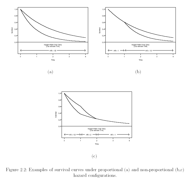
5	Weighted Logrank Statistics Generalization of statistics derived from the proportional hazards setting Particularly of interest in the setting of nonproportional hazards Early, transient treatment effects Late treatment effects occurring after some delay
6	Constant, Late, Early Effects
7	Right Censored Data Notation:
8	Logrank Statistic Originally described as a straightforward approach to the presence of censoring If we had followed all subjects a fixed amount of time, we could use binomial proportions or odds Time is merely a confounder and/or precision variable in the analysis of the probability of failure Adjust for time by stratification (dummy variables)
9	Logrank Statistic Analysis of stratified 2x2 contingency tables Mantel-Haenszel statistic Noninformative censoring allows the repeated use of the same people in all of the strata Can also be derived as the score statistic from the proportional hazards partial likelihood
10	Partial Likelihood
11	Partial Likelihood Based Score
12	Logrank Statistic Under proportional hazards, the efficient score statistic is a weighted average of differences in hazards (proportions) Weights are roughly proportional to the size of the risk sets at each failure time Intuitively reasonable if the treatment effect is constant over time Under time-varying treatment effects, we might want to weight more heavily the times with a difference in hazards
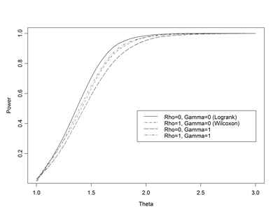
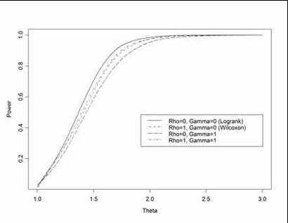
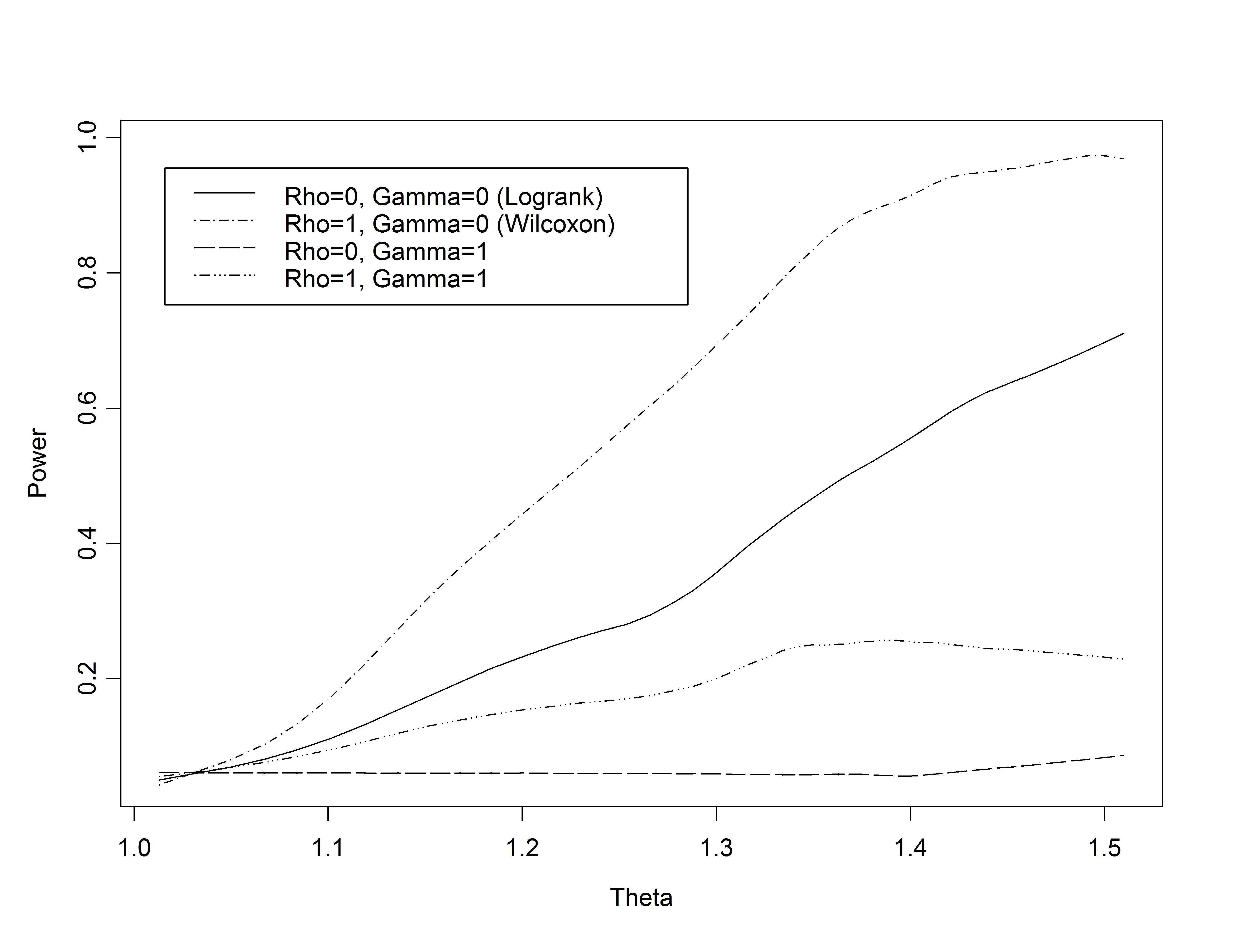
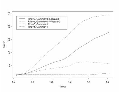
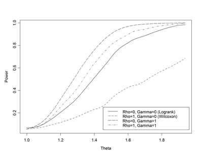
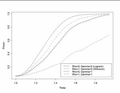
13	Weighted Logrank Statistics Choose additional weights to detect anticipated effects
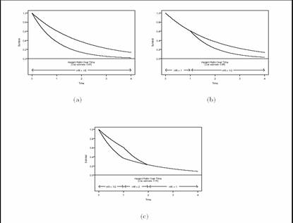
14	G^rg Family Fleming & Harrington: Logrank statistic: ρ=0; γ=0 Wilcoxon statistic: ρ=1; γ=0 Weights early differences more heavily “Early” defined relative to survivor function, not time ρ=1; γ=1 Places greatest weight between 25^th, 75^th quantiles ρ=0; γ=1 Weights late differences more heavily
15	Constant, Late, Early Effects
16	Constant (PH) Effects: Power
17	Early Effects: Power
18	Late Effects: Power
19	Caveats The scientific interpretation of these weighted logrank statistics is difficult in the presence of nonproportional hazards (And why use them when we have PH?) The weights we specify are only part of the story The size of the risk sets at each failure time also affects the inference
20	Other Factors Affecting Weights The size of the risk set is affected by The survivor function in each group Something we care about Something we hope is consistent across studies The censoring distribution in each group Something that we usually regard a matter of convenience Something that we hope will not affect the scientific estimates, just the statistical precision
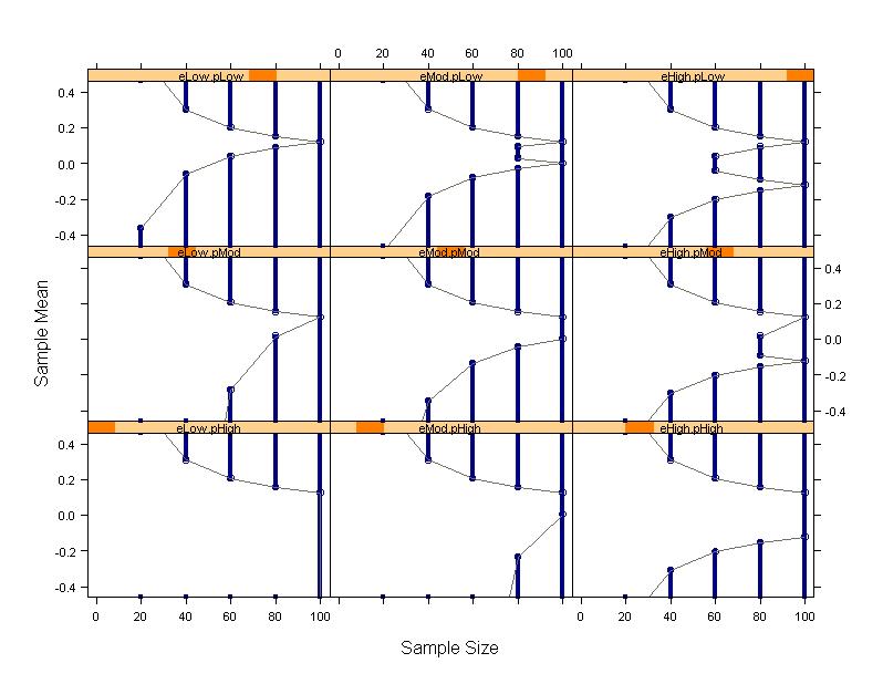
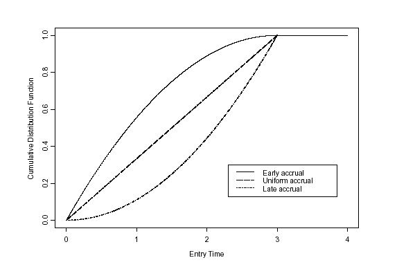
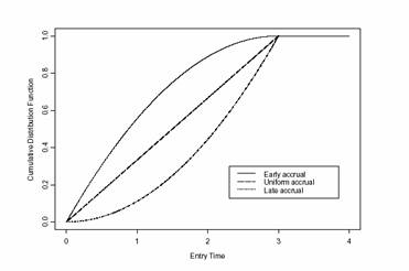
21	Censoring Affected By Accrual Consider patterns of accrual that are either uniform, faster early, or faster late
22	Inference for PH, Late Tx Effects
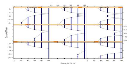
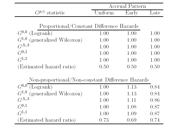
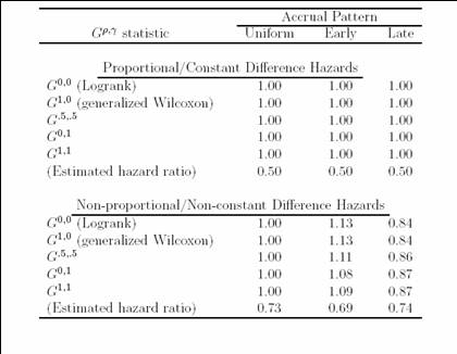
23	Effect of Censoring on Inference The estimates of treatment benefit can vary even more markedly according to the censoring distribution With “crossing hazards”, changes in censoring can make any of the weighted logrank statistics qualitatively differ from each other And it is possible for the conclusion drawn from the statistic to differ markedly from the conclusion suggested by the survival curves
24	Hypothetical Example: Setting Consider survival with a particular treatment used in renal dialysis patients Extract data from registry of dialysis patients To ensure quality, only use data after 1995 Incident cases in 1995: Follow-up 1995 – 2002 (8 years) Prevalent cases in 1995: Data from 1995 - 2002 Incident in 1994: Information about 2^nd – 9^th year Incident in 1993: Information about 3^rd – 10^th year … Incident in 1988: Information about 8^th – 15^th year
25	Hypothetical Example: KM Curves
26	Who Wants To Be A Millionaire? Proportional hazards analysis estimates a Treatment : Control hazard ratio of B: 1.13 (logrank P = .0018) The weighting using the risk sets made no scientific sense Statistical precision to estimate a meaningless quantity is meaningless
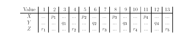
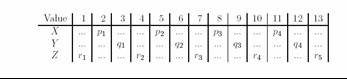
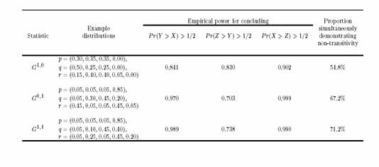
27	Transitivity The weighting scheme used in the weighted logrank statistics also introduces intransitivity to studies The weights are stochastically determined from Each group’s survivor function The censoring distribution Hence we can obtain A > B > C > A Very distressing to regulatory agencies, if not all scientists
28	Demonstrating Intransitivity
29	Sequential Clinical Trials Overview
30	Clinical Trials Experimentation in human volunteers Efficacy: Can the treatment alter the disease process in a beneficial way? Phase II (preliminary); Phase III Safety: Are there adverse effects that clearly outweigh any potential benefit? Phase I; Phase II Effectiveness: Would adoption of the treatment as a standard affect morbidity / mortality in the population? Phase III (therapy); Phase IV (prevention)
31	Collaboration of Multiple Disciplines
32	Statistical Planning Ensure that the trial will satisfy the various collaborators as much as possible Discriminate between relevant scientific hypotheses Scientific and statistical credibility Protect economic interests of sponsor Efficient designs; Economically important estimates Protect interests of patients on trial Stop if unsafe or unethical and when credible decision can be made Promote rapid discovery of new beneficial treatments
33	Address Variability At the end of the study Estimate of the treatment effect Single best estimate Precision of estimates Decision for or against hypotheses Binary decision Quantification of strength of evidence
34	Statistical Design: Sampling Plan Ethical and efficiency concerns are addressed through sampling which might allow early stopping During the conduct of the study, data are analyzed at periodic intervals and reviewed by the DMC Using interim estimates of treatment effect Decide whether to continue the trial If continuing, decide on any modifications to sampling scheme
35	Sampling Plan Perform analyses at sample sizes N₁. . . N_J Can be randomly determined At each analysis choose stopping boundaries a_j < b_j < c_j < d_j Compute test statistic T(X₁. . . X_N_J) Stop if T < a_j (extremely low) Stop if b_j < T < c_j (approximate equivalence) Stop if T > d_j (extremely high) Otherwise continue (with possible adaptive modification of analysis schedule, sample size, etc.)
36	Sampling Plan Issues when using a sequential sampling plan Design stage Boundaries to satisfy desired operating characteristics E.g., type I error, power, sample size requirements Monitoring stage Flexible implementation of the stopping rule to account for assumptions made at design stage E.g., sample size adjustment to account for observed variance Analysis stage Providing inference based on true sampling distribution of test statistics
37	Sampling Plan: Examples Alternative plans for a sepsis trial comparing 28 day mortality rates with 90% power to detect a 7% improvement using N=1700 Fixed sample study: Gather data on 1700 patients and analyze data Group sequential study (OBF efficacy, P=0.8 futility): Perform analysis after 425 patients If test statistic very low or very high, stop If test statistic intermediate, accrue another 425 Repeat, as necessary, until maximum of 1700 patients
38	Sampling Plan: Examples Advantage of stopping rule: Fixed sample: 4.18% improvement is significant Harmful: Power= 0.001; Average N= 1700 No effect: Power= 0.025; Average N= 1700 Low effect: Power= 0.500; Average N= 1700 Beneficial: Power= 0.975; Average N= 1700 Grp sequential: 4.24% improvement is significant Harmful: Power= 0.001; Average N= 785 No effect: Power= 0.025; Average N= 987 Low effect: Power= 0.477; Average N= 1330 Beneficial: Power= 0.966; Average N= 1104
39	Major Issue: Frequentist Inference Often, the criteria for judging statistical evidence in clinical trial results are based on frequentist criteria Experimentwise error probabilities Type I, II errors, power Optimality of point estimates Bias, mean squared error Computation of precision Confidence intervals
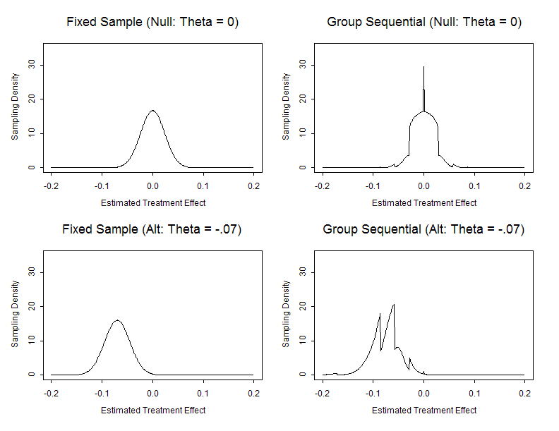
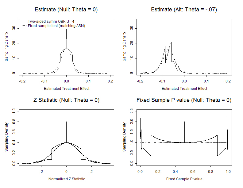
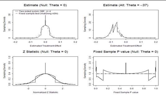
40	Major Issue: Frequentist Inference Frequentist operating characteristics are based on the sampling distribution Stopping rules do affect the sampling distribution of the usual statistics MLEs are not normally distributed Z scores are not standard normal under the null (1.96 is irrelevant) The null distribution of fixed sample P values is not uniform (They are not true P values)
41	Sampling Distribution of Estimates
42	Sampling Distribution of Estimates
43	Sampling with Stopping Rules
44	Operating Characteristics For any stopping rule, however, we can compute the correct sampling distribution with specialized software From the computed sampling distributions we then compute Bias adjusted estimates Correct (adjusted) confidence intervals Correct (adjusted) P values Candidate designs can then be compared with respect to their operating characteristics
45	Stopping Criteria: Boundary Scales Various test statistics are transformations A stopping rule for one test statistic is easily transformed to a rule for another statistic “Group sequential stopping rules” Sum of observations Point estimate of treatment effect Normalized (Z) statistic Fixed sample P value Error spending function Conditional probability Predictive probability Bayesian posterior probability
46	Unified Family: MLE Scale Boundary shape function unifies families of stopping rules Wang & Tsiatis (1987) based families O’Brien & Fleming (1979); Pocock (1977) Also used by Emerson & Fleming (1989); Pampallona & Tsiatis (1994) Triangular test (Whitehead, 1983) Seq cond probability ratio test (Xiong & Tan, 1994) Conditional or predictive power Peto-Haybittle (using Burington & Emerson, 2003)
47	Conditions for Early Stopping Down columns: Early vs no early stopping Across rows: One-sided vs two-sided
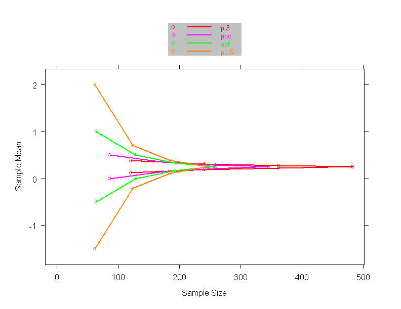
48	Boundary Shape Functions A wide variety of boundary shapes possible All of the rules depicted have the same type I error and power to detect the alternative
49	Evaluation of Designs Process of choosing a trial design Define candidate design Usually constrain two operating characteristics Type I error, power at design alternative Type I error, maximal sample size Evaluate other operating characteristics Different criteria of interest to different investigators Modify design Iterate
50	Operating Characteristics Generally the same for all stopping rule s Frequentist power curve Type I error (null) and power (design alternative) Sample size requirements Maximum, average, median, other quantiles Stopping probabilities Inference at study termination (at each boundary) Frequentist inference Bayesian inference under spectrum of priors Futility measures Conditional power, predictive power
51	Sequential Clinical Trials Time Varying Treatment Effects
52	Time Invariant Treatment Effects The design, monitoring, and analysis of sequential trials is fairly well established for treatment effects that do not vary over time Means Proportions Odds Proportional hazards
53	Nonproportional Hazards With nonproportional hazards, new issues must be addressed Choice of summary measure Handling any dependence on the censoring distribution Definition of alternative Computation of operating characteristics Flexible implementation
54	Censoring Distribution A summary measure that depends on the censoring distribution is the biggest problem In a survival study, we typically have a different censoring distribution at successive analyses Hence, different summary measures are being tested at different analyses
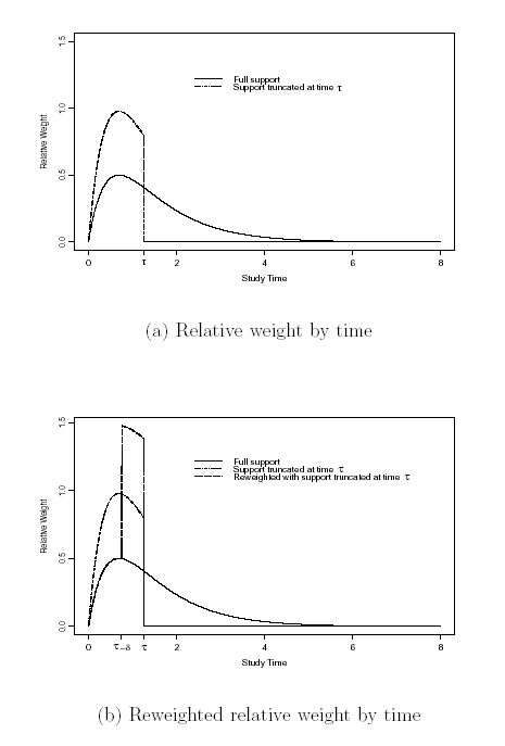
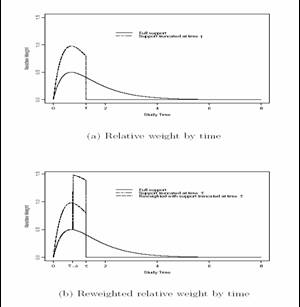
55	Weighted Logrank Statistics This is particularly true with weighted logrank statistics At the final analysis, weights will be applied over a wider range of time than is possible at earlier analyses At the earlier analyses, early results are weighted more heavily than they will be later
56	Example A 7 year trial is planned using a weighted logrank statistic to place weight late Plan: 1/28, 2/28, 3/28, …, 7/28 weight over the 7 years An interim analysis conducted after 3 years 1/6, 2/6, 3/6 over the first three years (later years have no data, hence no weights)
57	One Proposed Solution Apply weights due to be used late in study to the most longterm experience In the example, we would apply weights 1/28, 2/28, 25/28 Tends to (appropriately) inflate variability of statistic at interim analyses Intuitively reasonable in that the results for the longest observations should be more indicative of the future Similar to imputing future observations
58	Reassigning weights
59
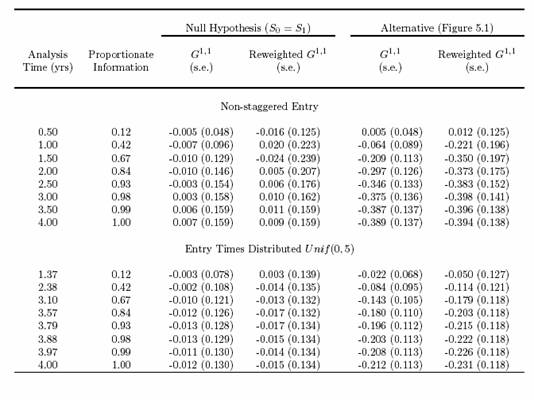
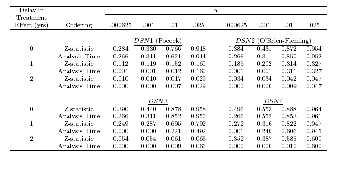
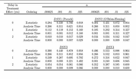
60	Inferential Methods Analysis at the end of the trial must take into account the sampling plan Methods for confidence intervals involve defining an “ordering of the sample space” Must decide how to order results obtained at different stopping times Previously described methods Analysis time or stagewise ordering MLE ordering Z statistic ordering
61	Optimality Criteria There is no single best ordering Whitehead and Jennison & Turnbull prefer the analysis time ordering In the presence of time invariant treatment effects, it does not usually make too much of a difference
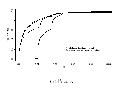
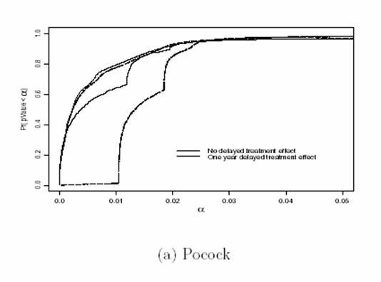
62	Optimality Criteria However, the analysis time ordering corresponds to the error spending function You can never get a P value less than the error spent This means that with late onset treatment effects, you can not achieve as low P values as might otherwise be indicated Great impact on “pivotal trials”
63
64	Power to Obtain Low P values
65	Final Comments We have found that our first attempts at improving the scientific use of the weighted logrank statistics has worked well Greatly improved consistent estimation Minimal loss of power
66	Final Comments Much more work is needed when using sequential methods with time varying treatment effects We are exploring the use of Bayesian random walk processes to model the types of alternatives that might be addressed However, this is truly an insoluble problem: There is nothing in the data that can guarantee what future data might look like
67	Final Comments In any case, however, the issue of paramount importance is that decisions about the summary measure be driven by the scientifically important effects Censored survival data requires a bit of extra care But the scientific issues are the same